Section 4a: Electrical Resistivity Surveying

Electrical and Electromagnetic Methods

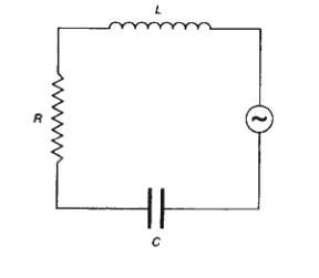
Electric circuit has three main properties:

• Resistance (R): resistance to movement of charge

• Capacitance (C): ability to store charge

• Inductance (L): ability to generate current from changing magnetic field arising from moving charges in circuit

Each electrical property is basis for a geophysical method:

Resistivity: measures apparent resistance of ground to direct current (DC) flow

Induced Polarisation: measures effect on current flow of charge storage in ground

Spontaneous Potential: measures naturally occurring DC currents

Electromagnetic Methods (EASC 307): measure apparent resistance of ground to induced alternating current (AC) flow

Resistivity Applications

• Resistivity methods first developed in early 1900s

• Used extensively in borehole logging for oil exploration from 1920s (Schlumberger)

• Surface resistivity in common use from 1970s in mineral and groundwater exploration

• Surface resistivity now used to monitor groundwater contamination, locate subsurface cavities and fissures

Resistance

Ohm’s Law

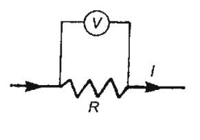
In an electrical circuit, the electrical resistance R of a wire in which current I is flowing is given by Ohm’s Law:

where V is potential difference across wire.

R is measured in ohms, V in volts, and I in amps.

Doubling length of wire or increasing its diameter changes the resistance.

Resistance is NOT a fundamental characteristic of the metal in the wire.

Resistivity

For a uniform wire or cube, resistance is proportional to length and inversely proportional to cross-sectional area

Constant of proportionality is called Resistivity r:

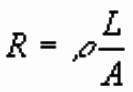
Resistivity r is the fundamental physical property of the metal in the wire

r is measured in ohm-m (check above definition)

Conductivity s is defined as 1/r, and is measured in Siemens per metre (S/m), equivalent to ohm^-1m^-1.

Non-Uniform Bodies

Effect of Geometry

If two media are present in cube with resistivities r₁and r₂, then both their proportions and their geometry determine the resistance of cube.

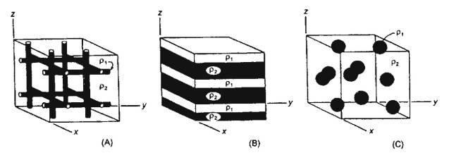
Apparent resistivity of above cubes is quite different even though two resistivities are the same.

Anisotropy

In a uniform cube, electrical properties are same in each direction and cube is said to be isotropic.

In a non-uniform cube, electrical properties can vary with direction, and cube is said to be anisotropic.

• Anisotropy found in platey structures

• Ratio of maximum to minimum resistivity is called coefficient of anisotropy, and is usually in range of 1-2.

Current Flow in Geological Materials

Electrical current can flow, i.e. electrical charges can move, in rocks and soils, but process is usually different from current flowing in a metal wire.

Three main mechanisms of current flow:

1) Electrolytic Conduction

• Occurs by relatively slow migration of ions in a fluid electrolyte.

• Controlled by type of ion, ion concentration, and ionic mobility.

2) Electronic Conduction (as in metal wire)

• Occurs in metals by rapid movement of electrons.

• Found in native metals and some metal oxides and sulphide ores

3) Dielectric Conduction

• Occurs in weakly conducting materials, or insulators, in presence of external alternating current

• Atomic electrons are shifted slightly relative to nucleus

In most rocks, DC current flow is by electrolytic conduction:

• controlled by pore fluid and pore geometry

• mineral grains of matrix contribute little, except if metal ore

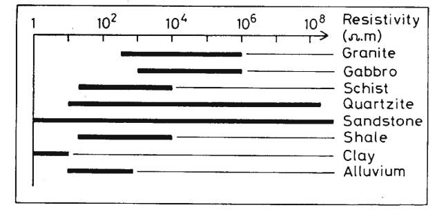
• geological materials show huge variation (10²⁴) in resistivities: 1.6 x 10^-8 for native silver to 1.6 x 10¹⁶ for pure sulphur

Archie’s Law

In sedimentary rocks, resistivity of pore fluid is probably single most important factor controlling resistivity of whole rock.

Archie (1942) developed empirical formula for effective resistivity of rock:

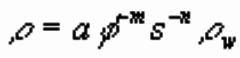
where f is porosity, s is the volume fraction of pores with water, and r_w is resistivity of pore fluid.

a, m, and n are empirically determined constants:

0.5<a<2.5

1.3<m<2.5

n ~ 2

r_w is controlled by dissolved salts and can vary between 0.05 ohm-m for saline groundwater to 1000 ohm-m for glacial meltwater.

• Archie’s Law ignores the effect of pore geometry, but is a reasonable approximation in many sedimentary rocks

• In granite, where porosity is due to fracturing law can break down

Common Resistivity Values

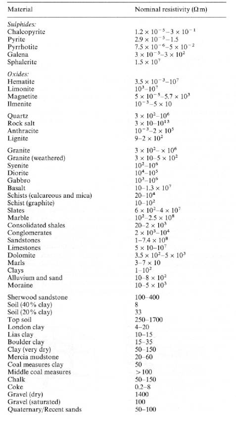
Common Resistivity Values (cont)

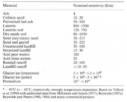
Range of Resistivities for Common Rock Types

Current Flow from One Electrode in a Uniform Earth

For single electrode planted in the Earth with circuit completed by another very distant electrode, current flow is radially symmetric.

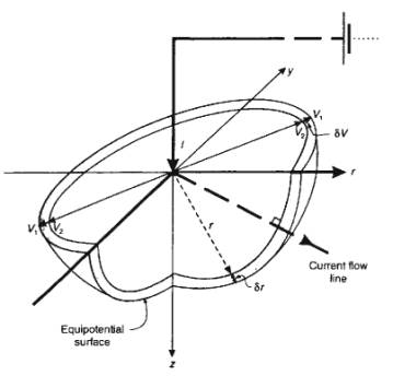
Current Density

If current I flowing into ground at electrode, that current is distributed over hemispherical shell. Current density J given by:

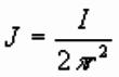
J decreases with increasing distance as current dissipates.

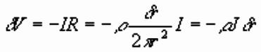
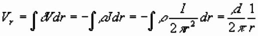
Voltage at Distance r

From Ohm’s Law applied to a hemispherical shell of radius r and thickness dr, voltage change across shell is given by:

So voltage (or potential) at distance r given by summing shells:

(V_r=0, inf)

Potential Difference with Two Electrodes

If second electrode is placed at B close to first electrode located at A, it affects current distribution and ground potential:

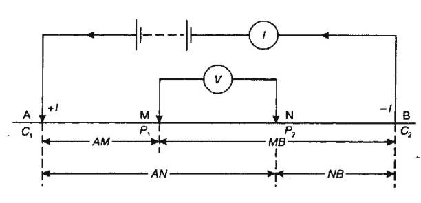
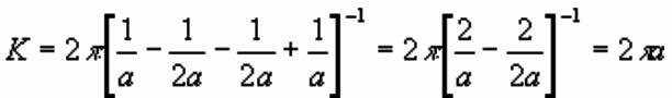
Potential at any point P in ground is equal to sum of potential from each electrode (c.f. work done going uphill by different paths):

For electrodes at M and N, can use single electrode expression:

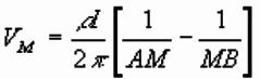
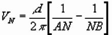
Actually measure differences in potential,. Between M and N is:

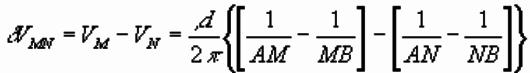
So resistivity of ground is:

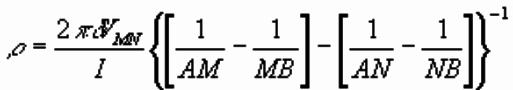
Resistivity given by measured voltage and electrode geometry

Current Flow in Uniform Earth with Two Electrodes

Current injected by electrode at S₁ and exits by electrode at S₂:

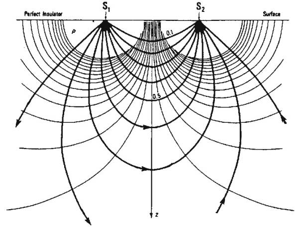
Lines of constant potential (equipotential) are no longer spherical shells, but can be calculated from expression derived previously.

Current flow is always perpendicular to equipotential lines.

• Where ground is uniform, measured resistivity should not change with electrode configuration and surface location

• Where inhomogeneity present, resistivity varies with electrode position. Computed value is called apparent resistivity r_A.

Depth of Current Penetration

Current flow tends to occur close to the surface. Current penetration can be increased by increasing separation of current electrodes.

Proportion of current flowing beneath depth z as a function of current electrode separation AB:

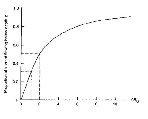
Example

If target depth equals electrode separation, only 30% of current flows beneath that level.

• To energise a target, electrode separation typically needs to be 2-3 times its depth.

• High electrode separations limited by practicality of working with long cable lengths. Separations usually less than 1 km.

Electrode Configurations and Geometric Factors

The general expression for resistivity derived previously, which in practice is the apparent resistivity, can be written as:

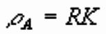
where R is a resistance term given by R=dV/ I and K is given by:

K is called the geometric factor for the electrode array.

Electrode Arrays

• An electrode array consists of two electrodes at which DC current flows into and out of the ground plus two electrodes between which the potential difference at the surface is measured .

• The apparent resistivity measured by different arrays is not the same, because the geometric factor K is different.

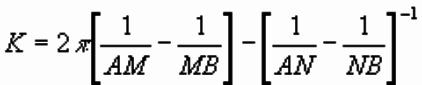
Example

Suppose current and potential electrodes are equally spaced. Then K simplifies to:

This type of array is called a Wenner Array invented in 1912

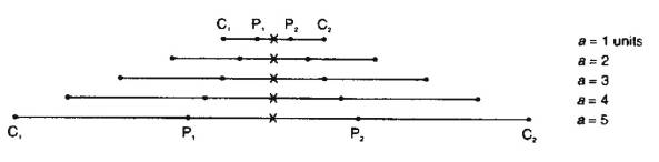
Common Electrode Arrays

• Below are electrode arrays most commonly used in resistivity

• C are current electrodes and P are potential measurement electrodes. X is location assigned to measurement.

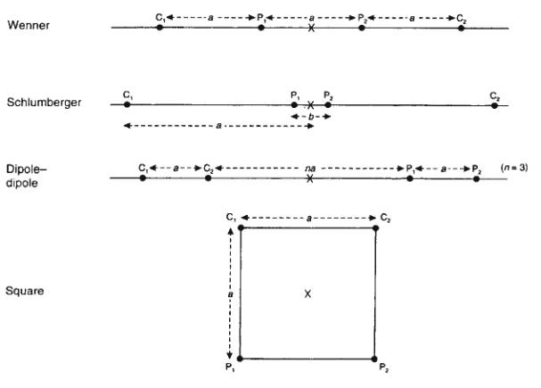
Geometric Factors and Apparent Resistivities

Wenner Array

Schlumberger Array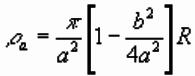

Dipole-Dipole

Square

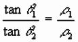
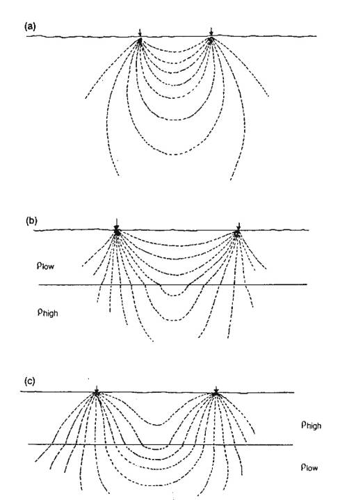
Properties of Different Electrode Arrays

Different subsurface current flow from different electrode arrays.

Relative contributions from subsurface to measured potential for different electrode arrays (dashed lines negative):

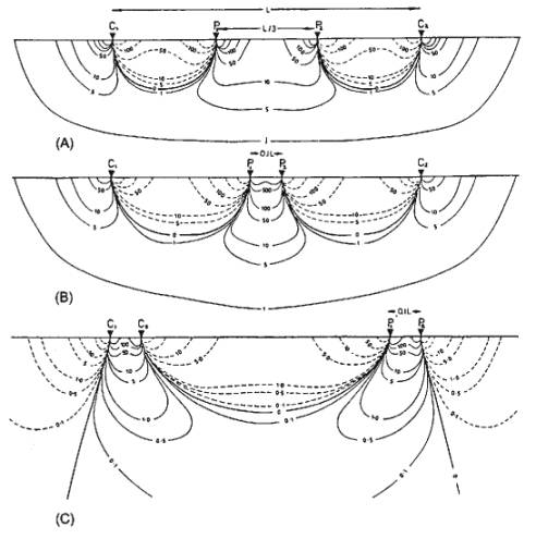
A. Wenner: Alternating +ve and –ve near-surface regions cancel, and main response is from depth, which is fairly uniform laterally. Good for determining depth variations in 1-D Earth.

B. Schlumberger: Equivalent vertical resolution to Wenner (distance between contours), but deep response is concave upwards. More sensitive to lateral variation in Earth.

C.Dipole-Dipole: Poor vertical resolution as contours spaced widely. Lobes from each dipole penetrate deeply indicating good sensitivity to lateral variation at depth.

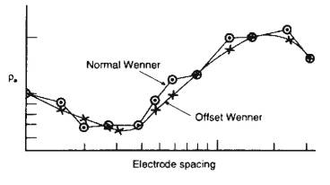
Offset Wenner Array

Wenner array often offset to repeat reading. Average value used.

Example

Consider buried sphere with resitivity of 100 ohm-m.

• When sphere in area of positive signal contribution, measured apparent resistivity is 91.86 ohm-m.

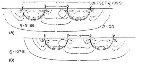
• When sphere in area of negative signal contribution, measured apparent resistivity is 107.81 ohm-m.

• Average of two readings is 99.88 ohm-m.

• Example of reduced error: Offset Wenner curve is smoother.

Current Flow in Layered Media

More realistic to consider vertical layers, for example water saturated horizontal aquifer.

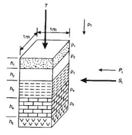
Current flowing vertically through layers will traverse each in series, like resistors connected in series in an electrical circuit. Transverse resistance given by:

Current flowing laterally will tend to take path of least resistance, and layers will behave as resistors connected in parallel. Longitudinal conductance given by:

Problem is that measured resistivity is a function of both layer resistivity and layer thickness, and both cannot be easily resolved.

Example

5-m thick layer with resistivity of 100 ohm-m, has same lateral resistivity as 10-m thick layer with 200 ohm-m resistivity.

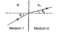
Refraction of Electrical Current

In a uniform Earth with no boundaries, with two widely separated electrodes (one at infinity), current flow is radially symmetric.

If nearby boundary, current flow is deviated: away from more resistive medium, towards more conductive one.

Current flow refracts at boundary in proportion to change in resistivity:

Example of Current Flow in Two Layer Medium

Have already found direction of current flow between two electrodes in uniform medium:

In two layer medium, current travels preferentially in low resistivity medium.

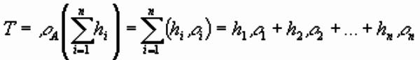
Method of Images

Potential at point close to a boundary can be found using "Method of Images" from optics.

In optics:

Two media separated by semitransparent mirror of reflection and transmission coefficients k and 1-k, with light source in medium 1.

• Intensity at a point in medium 1 is due to source and its reflection, considered as image source in second medium, i.e source scaled by reflection coefficient k.

• Intensity at point in medium 2 is due only to source scaled by transmission coefficient 1-k as light passed through boundary.

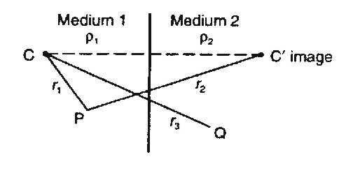
Electrical Reflection Coefficient

In electrical current flow:

Consider point current source and find expression for current potentials in medium 1 and medium 2:

Use potential from point source, but 4p as shell is spherical:

Potential at point P in medium 1:

Potential at point Q in medium2:

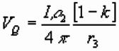
At point on boundary mid-way between source and its image:

r₁=r₂=r₃=r say. Setting V_p = V_q, and cancelling we get:

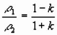
Solving for k:

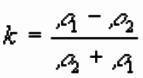
k is electrical reflection coefficient and used in interpretation

Practical Resistivity Surveys

By Ohm’s Law we need to measure the current that flows into the ground and the potential difference at various surface locations.

Need high resistance in potential measuring circuit to avoid short circuiting ground: most commercial systems have >1Mohm.

Problems:

• With DC currents, anions build up around anode (+ve electrode), and cations around cathode (-ve electrode).

• Telluric currents, naturally occurring currents, flow in Earth and create regional potential gradients that confuse readings.

• Cable lengths also restrict surveys, particular for deep objectives where electrode separations must be large

Solutions:

• Use very low frequency AC alternating current to reduce ion buld up: anode and cathode are switched repeatedly.

• Average measurement over several cycles, so effects of telluric currents and anion buildup tend to cancel.

Complication:

Depth of penetration changes with AC frequency, so need to select appropriate value for survey:

· 10 m deep target requires ~100 Hz

• 100 m deep target requires ~10 Hz

Two Main Survey Methods:

Vertical Electrical Sounding: Depth variation in resistivity

Constant Separation Traversing: Lateral variations in resistivity

Vertical Electrical Souding (VES)

Increasing distance between current electrodes increases depth of current penetration into Earth.

Vertical Electrical Sounding (r_a vs. depth)

Measurements are repeated as array is expanded about a fixed point, maintainng the relative spacing of the electrodes.

Used to find overburden thickness, aquifers and other horizontal structures

Wenner:

• All four electrodes have to be moved for each measurement

Schlumberger:

• Potential electrodes are kept fixed until measured voltage decreases to low values as potential gradient in ground falls with increasing current electrode separation.

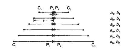
• Then moved and process repeated.

Dipole-Dipole and Square:

• Rarely used for VES surveys

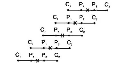
Constant Separation Traversing (CST)

Constant Separation Traversing (r_a vs. lateral distance)

Measurements are repeated as array is moved along a profile with electrodes maintained at fixed distances.

Used to detect shear zones, faults and other vertical boundaries

• In practice, acquisition can be simplified by laying out more than four electrodes, and using a subset for the reading.

• While reading made, electrodes can be moved from back to front of line to speed up acquisition.

Example

With 12 electrodes at 5 m intervals:

• Record Wenner array of 10 m spacing (distance between adjacent electrodes) using alternating electrodes.
• 5 m station spacing along profile.

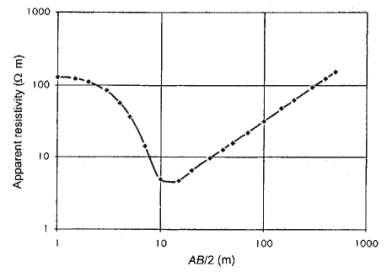
Examples of Resistivity Data

Vertical Electrical Sounding

Apparent resistivity usually plotted on logarithmic scale against electrode half-separation

Constant Separation Traversing

Resistivity values plotted on linear scale against location of centre of array along profile.

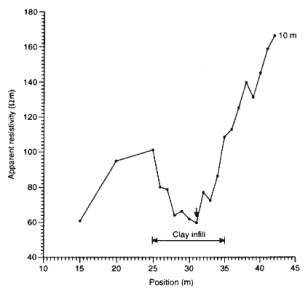
• Clay filled (more conductive) dissolution feature in limestone

Qualitative CST Interpretation: In-Line Array

As array moves toward lower resistivity medium, current flow lines converge on interface:

i. Current density increased at boundary, but decreased at potential measurement electrodes, so r_a falls.

ii. r_a falls until C₂ at boundary when r_a reaches a minimum

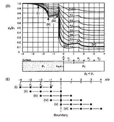
iii. When C₂ crosses boundary, current density increases close to boundary in medium 2, and is at a maximum when first potential electrode reaches boundary

iv. When entire array has crossed boundary, current density highest in resistive medium, and r_a falls sharply at potential dipole.

v. When C₂ crosses boundary, current density deflected from medium 1, increasing potential gradient slightly at potential dipole.

Qualitative CST Interpretation: Cross-Line Array

If array is oriented perpendicular to profile, current flow changes smoothly, and cusps in r_a curve do not occur.

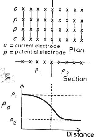
r_a varies smoothly from resistivity of medium 1 to value of medium 2

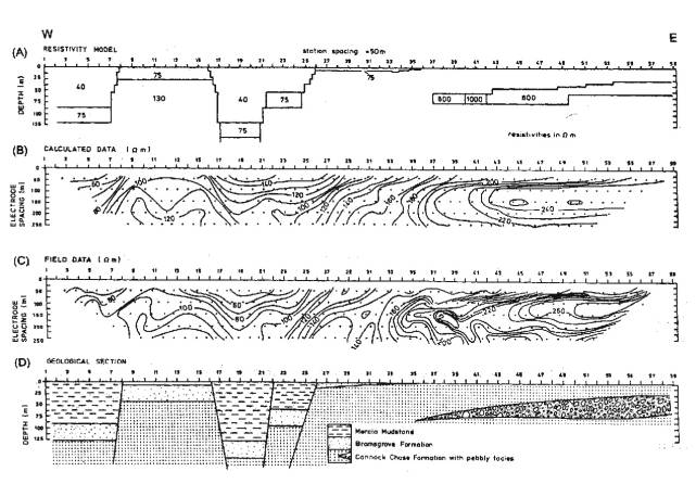
Qualitative CST Interpretation: Pseudosections

A single CST survey produces a profile of r_a vs. distance.

Increasing the electrode separation, increases depth of penetration.

Repeating the same profile with different electrode spacing, allows construction of a pseudosection of apparent resistivity.

Pseudosection is constructed by plotting measured value at intersection of lines drawn at 45^o from current and potential dipoles, and contouring result. (Discussed in detail in IP section)

Vertical axis is electrode spacing NOT depth, but does give a very approximate idea of the depth variation of r_a

Example of Pseudosection (Faulted Bedrock, UK)

Qualitative VES Interpretation: Two Layers

Basic Idea: Can consider current flow to refract in subsurface at layer boundaries, like light at a boundary.

Two Layer Earth

Consider Wenner array over two layer Earth:

Depth of current penetration increases with electrode separation a

For small a:

Current flows almost entirely in layer 1: r_a ~ r₁

As a increases:

Current flow lines reach interface, and are refracted towards interface as less resistive path is more attractive to current.

r₁ > r_a > r₂

For large a:

Almost all current flows in lower less resistive layer: r_a ~ r₂

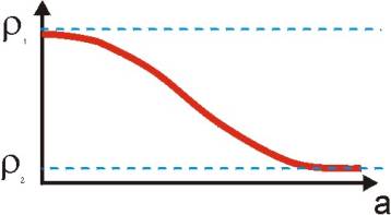
Only two possibilities in two layer case: r_a increases or decreases

Qualitative VES Interpretation: Three Layers

In three layer case, more variations in sounding curves exist

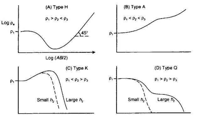
1. First part of curve at small electrode separations can be analysed as two layer case to see if r_a increase or decreases into second layer.

2. Comparing curve at small and large spacings indicates resistivity of lower layer relative to upper.

3. Character of mid-part of curve indicates nature of middle layer:

• Types H & K have distinct maximum/minimum and indicate anomalously high/low resistivity respectively.

• Types A & Q show steady change indicating middle layer has r intermediate between upper and lower layer

Layer only shows up in curve if it is sufficiently thick, and resistivity sufficiently different from others, e.g. D with small h₂.

Qualitative VES Interpretation: Four Layers

Many more combinations possible in four layer case

Two Examples:

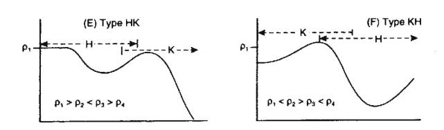
• In general, number of detectable layers equal to number of turning points in sounding curve plus one.

• Turning point due to interface, so number of layers is one greater.

• Electrode separation, at which turning points occur, has no connection with depth to interface.

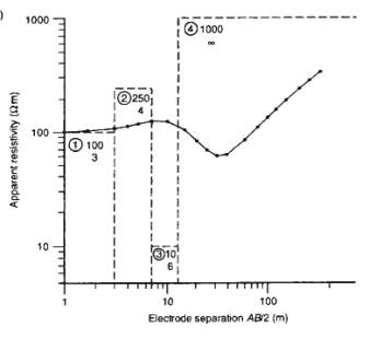
Example: Interface location plotted on electrode separation axis

Quantitative VES Interpretation: Master Curves

Layer resistivity values can be estimated by matching to a set of master curves calculated assuming a layered Earth, in which layer thickness increases with depth. (seems to work well)

For two layers, master curves can be represented on a single plot

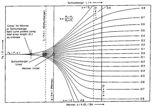
Master curves: log-log plot with r_a / r₁ on vertical axis and a / h on horizontal (h is depth to interface)

• Plot smoothed field data on log-log graph transparency.
• Overlay transparency on master curves keeping axes parallel.
• Note electrode spacing on transparency at which (a / h=1) to get interface depth.
• Note electrode spacing on transparency at which (r_a / r₁ =1) to get resistivity of layer 1.
• Read off value of k to calculate resistivity of layer 2 from:

Quantitative VES Interpretation: Inversion

Curve matching is also used for three layer models, but book of many more curves.

Recently, computer-based methods have become common:

• forward modelling with layer thicknesses and resistivities provided by user
• inversion methods where model parameters iteratively estimated from data subject to user supplied constraints

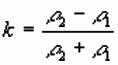
Example (Barker, 1992)

Start with model of as many layers as data points and resistivity equal to measured apparent resistivity value.

Calculated curve does not match data, but can be perturbed to improve fit.

Application to Bedrock Depth Determination

Both VES and CST are useful in determining bedrock depth

• Bedrock usually more resistive than overburden

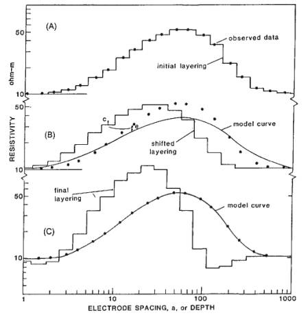
Example (South Wales)

For sewer construction wanted to avoid having to blast into sandstone bedrock.

CST profiling with Wenner array at 10 m spacing and 10 m station interval used to map bedrock highs

• Location where bedrock close to surface shown by CST profile.

• Depth to bedrock determined at specific locations by VES survey.

Application to Location of Permafrost

Permafrost represents significant difficulty to construction projects due to excavation problems and thawing after construction.

• Ice has high resistivity of 1-120 Mohm-m

Example (Fairbanks, Alaska)

Need to identify permafrost prior to construction of road cutting

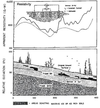
• Dashed line data acquired in spring are dashed line

• Solid line is data acquired in autumn and has lower resolution due to layer of thawed ground.

Application to Landfill Mapping

Resistivity increasingly used to investigate landfills:

• Leachates often conductive due to dissolved salts

• Landfills can be resistive or conductive, depends on contents

Example (Yorkshire, UK)

VES survey carried out over landfill. Resistivities in ohm-m.

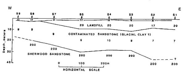
Three/Four layer VES analyses made at each sounding location depending on shape of r_a curve.

Results plotted side by side to constuct 2-D model of landfill.

• Landfill shows as 10 m thick layer with 20 ohm-m resistivity

• Bedrock shows as much higher 200 ohm-m layer

• Contaminated sandstone beneath landfill seen as anomalously low resistivity layer with value of ~9 ohm-m.